Simulation Workbench
The Simulation Workbench can be available and accessed based on the acquired license. If you have already purchased the corresponding license, you can find this workbench on the Workbenches Bar within SimLab Composer GUI.
- Simulation Toolbar
- Solids Menu
- Simulation Trees
- Links Menu
- Simulation Menu
- Interactive Menu
- Co-Simulation
Simulation Toolbar

SimLab Composer can be used to model the behavior of objects in 3D space. Using its powerful physics engine to allow simulation of the way bodies of many types are affected by a variety of physical stimuli, provided to simulate physical systems such as Rigid Body Dynamics in real-time and considering collision detection. The Simulation Workbench is dedicated to executing physical and mechanical simulations within the SimLab Composer application.
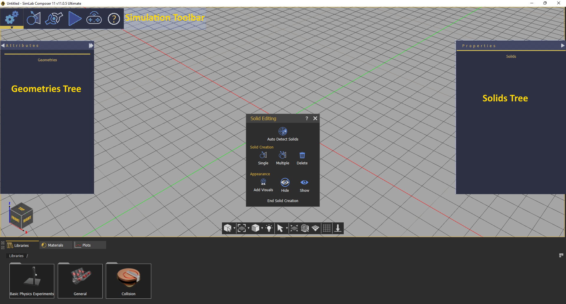
The image below shows the workspace of the Simulation Workbench, where the Solid Editing panel is active by default. The workspace presents the Simulation toolbar, the Geometries Tree, Solids Tree grouped with the Links Tree.
The Geometries Tree only appears in Solid Editing mode (When the Solid Editing dialog is open).
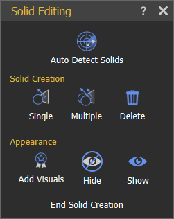
Simulation toolbar menus:
Check this mechanical simulation video
Solids Menu
To create a simulation the first step is to convert the 3D design to solid parts that can be physically simulated. This can be done either manually by selecting the parts and converting them to solids, or by clicking on Auto Detect Solids which will automatically detect the objects in the scene and convert them to solids.
- Auto Detect Solids
- Solid Creation
- Appearance
The Geometries Tree and the Models Library are associated with the Solids Tab. Once the Solids Tab is activated, they will be displayed on the left side and bottom of the application window, respectively.
Auto Detect Solids
Automatically identify and classify a model's geometries and assemblies into solids, by running an algorithm, where each solid contains either one geometry/assembly or a group of geometries/assemblies.
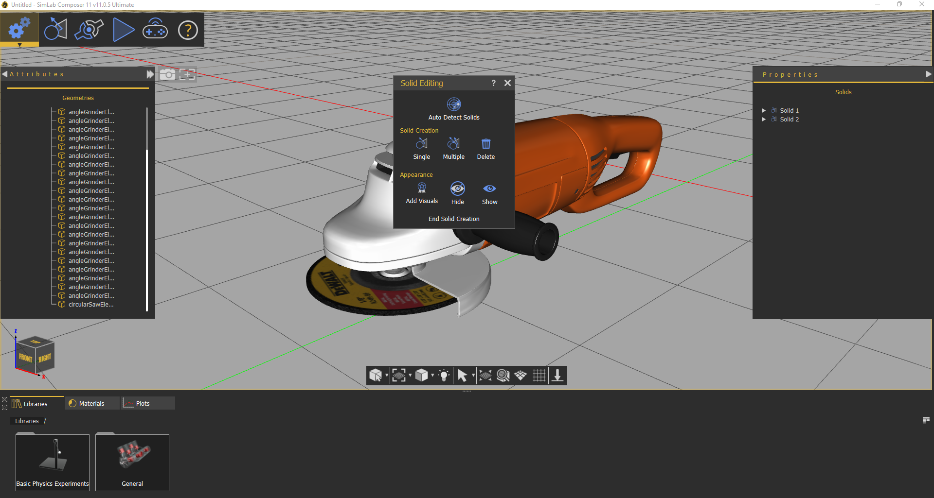
In the image below, the simulation workspace with an imported model is shown. Solids in the model has been detected and shown in the Solids Tree.

If the imported model is from an analytical file format like STEP, this algorithm makes use of the solids hints already embedded in an object to identify it as a solid.
In some cases, the automatic detection method may not yield the required results, the manual method for creating solids gives the user more control over solid creation.
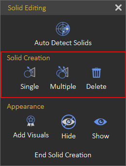
Solid Creation
Sometimes more control over solids creation may be needed. So rather than using the automatic detect function, Solid Creation section functions in the Solid Editing dialog are needed.
- Single: Manually creates a solid from the selected geometries or assemblies, geometry or an assembly can be selected either using the Geometries Tree or from the 3D Area. Multiple geometries can be selected from the Geometry Tree by holding the Ctrl key on the keyboard and clicking the desired geometries, then pressing the Create Solid button in order to create the desired solid. After clicking the Single button, only one solid will be created and all of its corresponding geometries will disappear from the Geometry Tree and move to the Solids Tree.
- Multiple: Manually create solids from selected geometries or assemblies. After clicking the Multiple buttons, multiple solids will be created and all of the corresponding geometries will disappear from the Geometry Tree and move to the Solids Tree.

Appearance
Sometimes, you may want a certain object to inherit the movement of a specified solid without including it in the equations of motion used by the corresponding solver, here the Manipulation Toolbar comes in handy. You find only one button in the Manipulation Toolbar, as shown in the following image:
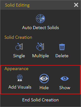
Add Visuals
Attaches selected geometry to an existing solid as a visualization object for visualization purposes that are not included in the simulation calculations. To add visuals, select the desired object(s) from the Geometry Tree, then click the Add Visuals button. Once it is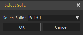 clicked, the Select Solid dialog box appears for the user to select the desired solid to attach visuals.
A solver is a component in SimLab Composer. SimLab Composer provides a library of solvers, each of which determines the time of the next simulation step and applies a numerical method to solve the set of equations that represent the model.
The Visual Icon appears next to the visual object's name in the Solids Tree. You can toggle this icon to turn it back as a normal object combined with the solid.
Visual elements can be disabled or enabled in the Solids Tree only if the Solids Tab is activated.
Hide / Show
This tool makes work easier while creating solids in complex models. It is considered a handy tool while working in simulation, where the user can hide/show objects in the 3D area.
Simulation Trees
There are three kinds of tree views in the Simulation Workspace:
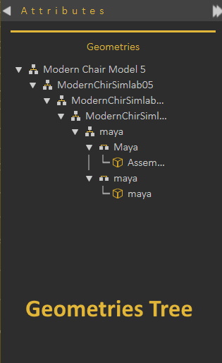


Geometries and Solids Trees
Both Trees show a hierarchical outline view of geometries and solids existing in the scene. Each geometry/solid branch or node can have a number of subitems, this is often visualized by an indentation in a list. A geometry/solid can be expanded to reveal subitems, if any exist, and collapsed to hide subitems. Geometries/Solids Trees allow the user to easily manage and navigate objects in them.
In the image below, the Geometries Tree is shown located at the left side of the application window, and the Solids Tree is at the right side. Both trees will appear when the Solid Editing dialog is open. Solids are included in the simulation calculations, while geometries are not. Using the functions in the Solid Editing dialog, a user can transfer objects from one tree to the other.

Links Tree
When the Solid Editing dialog is closed, the geometries tree will be hidden, and the Links Tree will appear grouped with the Solids Tree. It is a graphical control element that presents a list of created links connecting solids in the scene. Selecting a link in the tree will display its properties in the Attributes dialog on the left for the user to edit.
Models Library
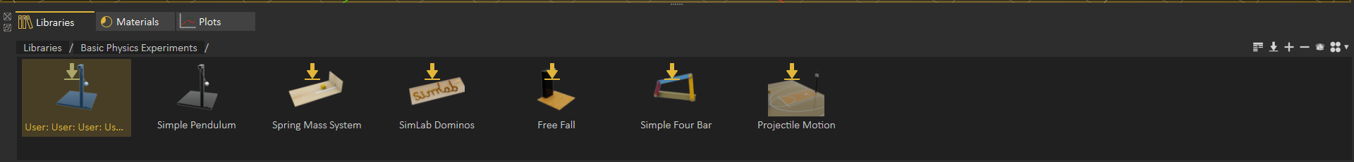
The Models Library acts as a container for pre-installed simulation models that come with the Simulation Edition of SimLab Composer, distributed into three groups: Basic Physics Experiments, General, and Collision (as shown in the following image). It is located at the bottom of the Solids workspace. You can choose any model of the provided sample just to run it as it is or edit it as you wish.
The toolbar of the Models Library is located horizontally on its right side:
- Manage Library: Launches Manage Library dialog that gives the user options to create, delete and rename model groups which are presented by tabs.
- Download Contents: This task is the same as in the Material Panel described in Navigator Panel.
- Add New: Allows the user to add newly created simulation models to any activated model tab within the Models Library.
- Delete Item: This command discards the selected model from the panel of the activated tab.
- Share Contents: This task is the same as in the Material Panel described in Navigator Panel.
- Change View: This task is the same as in the Material Panel described in Navigator Panel.
The Models Library is only associated with the Solids tab, it appears once the Solids tab is activated. By default, it also appears when you switch to the Simulation workbench.
Links Menu

The Lock Icon is different in the simulation. Locking an object makes it invulnerable to any external force.
Joints Group
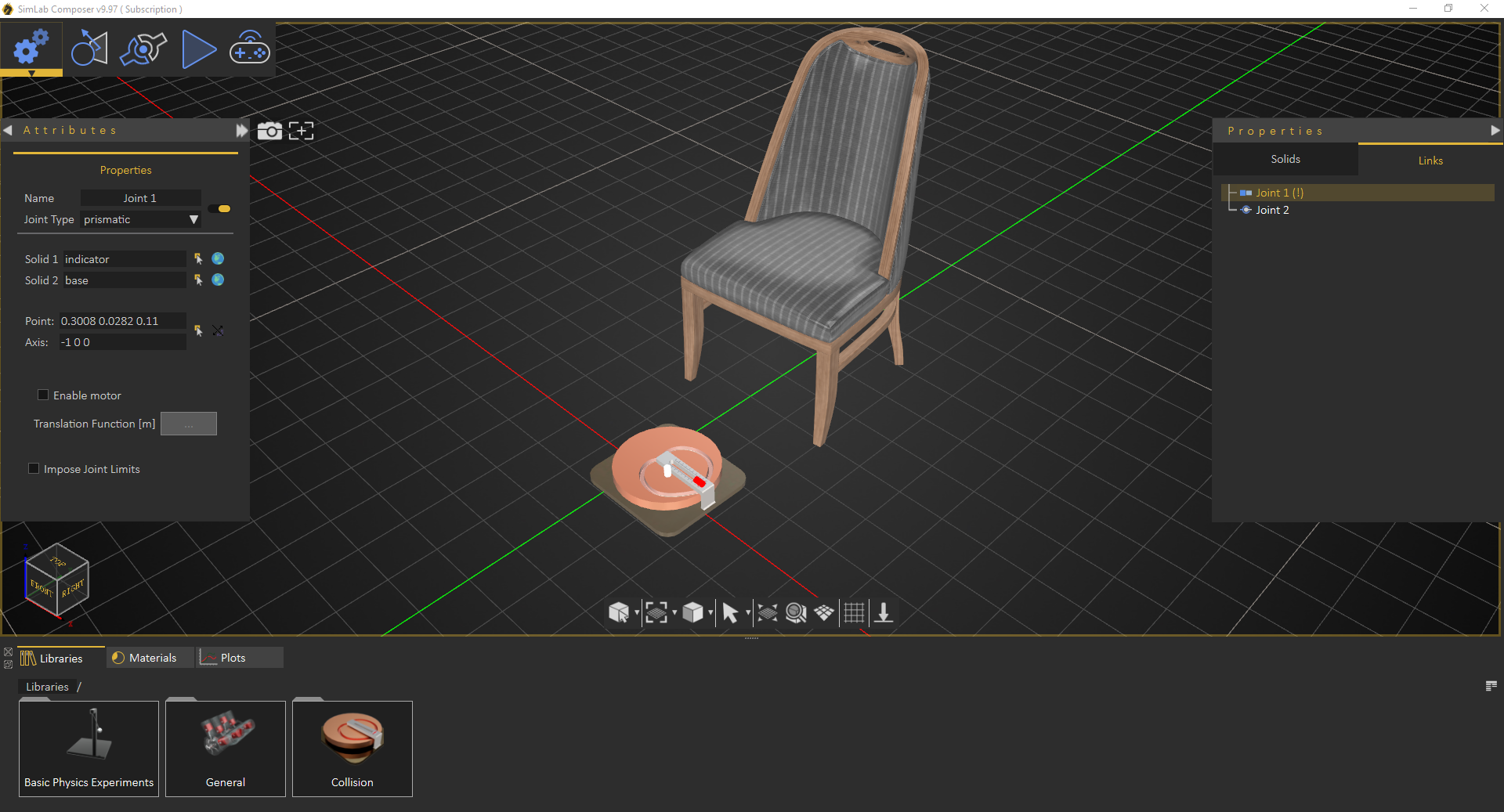
A joint is something like a hinge, which is used to connect two solids. It is a relationship that is enforced
between two bodies so that they can only have certain positions and orientations relative to each other. To create a joint between two solids, choose the joint type from the Links Menu, the joint will be added to the Links Tree, and its properties will appear in the Properties Panel on the left.
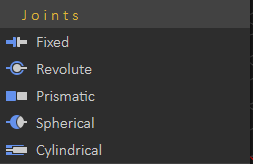
- Fixed: Maintains a fixed relative position and orientation between two solids, in practice, using this joint is rare. If two bodies are needed to be glued together, it is better to represent them as a single solid when deciding that both of the solids hold the same properties during the simulation session.
- Revolute: Also called pin joint, is a one-degree-of-freedom kinematics pair used in mechanisms. Revolute joints provide a single-axis rotation function used in many places such as door hinges, folding mechanisms, and other uni-axial rotation devices.
- Prismatic: Also called slider joint, provides a linear sliding movement between two bodies. The two joined solids have their rotation held fixed relative to each other, and they can only move along a specified axis, chosen by the user while specifying the joint properties.
- Spherical: Also called a ball and socket joint, is a joint in which the ball-shaped surface of a solid fits into the cup-like indentation of another solid. This type of joint allows the solid to move at a 360-degree angle—with more freedom than other joints.
- Cylindrical: A two-degrees-of-freedom kinematics pair used in mechanisms. Cylindrical joints provide a single-axis sliding function as well as a single-axis rotation, providing a way for two rigid bodies to translate and rotate freely.
A selected Joint requires its properties to be set in order to work appropriately.
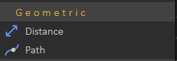
Geometric Group
The Geometric group is concerned with shape, size, the relative position of solids, and the properties of 3D space. Considers questions of relative position or spatial relationship of geometric figures and shapes.
- Distance: Creates a link between two solids based on maintaining a certain distance between them at all times during the simulation.

- Path: Specify a path in the scene for the solid to follow during the simulation
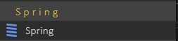
Spring Group
Creates a spring link between two points that the user selects. A spring is an elastic object used to store mechanical energy. The user needs to input the properties of the spring in the Properties dialog, Spring Constant, Damping, and Resting Length in order to work properly.
 Check this tutorial for more about spring creation and simulation.
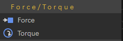
Force/Torque Group
A user can affect the behavior of a certain solid by applying an external force or torque on it.
- Force: Applies an influence (push or pull) that tends to change the motion of an object
including to begin moving from a state of rest, i.e. to accelerate. In other words, a force can cause an object with mass to change its velocity. A force has both magnitude and direction.
- Torque: applies an influence that produces a change in the rotational speed of an object.

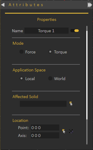
- Name: Where the user specifies a name for the new force or torque.
- Mode: This section allows the user to change between force and torque modes.
- Application Space: The user specifies whether the force or torque will follow the affected solid as it moves (Local), or stay static on the original point of application (World).
- Affected Solid: Where the user selects the affected solid.
- Location: Where the user selects the application point and axis for force or torque, in addition to that the ability to flip the force or torque direction.
- Magnitude Function: This edit button, if clicked, displays the Function Editor dialog box where the user specifies and selects the desired magnitude function for force or torque.

- Motion Function: Constant, Ramp, 3-4-5 Polynomial, Polynomial, Sine, Derivative, Integration, or Sequence.
- Constant.
- Ramp: Initial Value and Slope.
- 3-4-5 Polynomial: Amount of Displacement and Duration of Motion.
- Polynomial: C0, C1, C2, C3, C4, and C5.
- Sine: Amplitude, Phase, and Frequency.
- Derivative: Choose Function.
- Integration: Choose Function, Constant (C0), Lower Limit (X1), and Upper Limit (X2).
- Sequence: Select Sequence.
Gears Group
Gears group is located on the Links menu. You find two buttons in this group, as shown in the image. A brief description of each button, supported by the SimLab Composer's simulation engine, is given as follows:
- Gear (Gear Train or Transmission): Two or more gears working in a sequence. Such gear arrangements can produce a mechanical advantage through a gear ratio and thus may be considered a simple machine. Geared devices can change the speed, torque, and direction of a power source. The most common situation is for a gear to mesh with another gear.
- Rack and Pinion: A gear can also mesh with a non-rotating toothed part, called a rack, thereby producing translation instead of rotation. A rack is a toothed bar or rod that can be thought of as a sector gear with an infinitely large radius of curvature. Torque can be converted to linear force by meshing a rack with a pinion: the pinion turns; the rack moves in a straight line. Such a mechanism is used in automobiles to convert the rotation of the steering wheel into the left-to-right motion of the tie rod(s). Racks also feature in the theory of gear geometry, where, for instance, the tooth shape of an interchangeable set of gears may be specified for the rack (infinite radius), and the tooth shapes for gears of particular actual radii are then derived from that. The rack and pinion gear type is employed in a rack railway.
Pulley Group

- Pulley: A pulley may also be called a sheave or drum and may have a groove between two flanges around its circumference. The drive element of a pulley system can be a rope, cable, belt, or chain that runs over the pulley inside the groove.
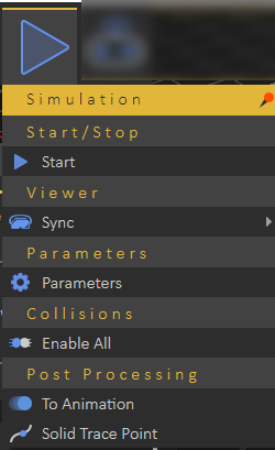
Simulation Menu
- Start/Stop
- Parameters Menu
- Collisions
- Post Processing

Start/Stop
Parameters

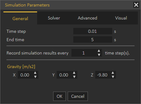
- Time Step: This numerical field is used by the chosen solver to determine the time step (in seconds) between iterations, reducing this value often produces more accurate results, but this requires executing additional calculations that affect the simulation speed and the size of the generated data. The default value is 0.001.
- End time: This numerical field tells the selected solver at which time (in seconds) the simulation will be stopped. Its default value is 10.
- Recording Simulation Results: This numerical field is used to ignore storing parts of the simulation data, and only saves data at a point after each interval specified (in time steps) by the user. It is usually used when the time step is very small, and the resulting data is very large. Its default value is 1.
- Gravity: X, Y, and Z: Specify (in m/s2: meter per second squared) the gravitational acceleration in X, Y, and Z directions. The default values are 0, 0, and -9.80, respectively.
- The Solver Tab includes the following setting fields, as shown in the following image:
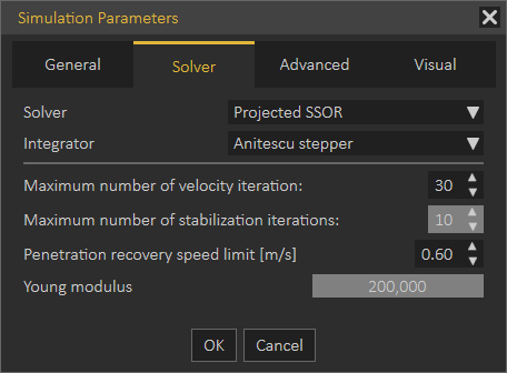
- Solver: Projected SSOR, Projected MINRES and DEM. (the default solver is Projected SSOR)
- Integrator: Anitescu Stepper and Tasora Stepper (the default integrator is Anitescu Stepper)
- Maximum Number of Velocity Iteration: (the default value is 30)
- Maximum Number of Stabilization Iteration: Only associated with the Tasora Stepper Integrator. (the default value is 10)
- Penetration Recovery Speed Limit: Only associated with the Anitescu Stepper Integrator (in m/s: meter per second) (the default value is 0.6)
- Young Modulus: Only associated with the DEM Solver, only enabled if the DEM Solver is chosen. (the default value is 200000)
- The Advanced Tab includes the following setting fields, as shown in the following image:
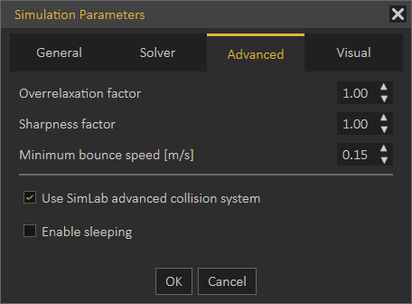
- Overrelaxation Factor: This option is associated with the Projected SSOR solver (the default value is 1)
- Sharpness Factor: This option is associated with the Projected SSOR solver (the default value is 1)
- Minimum Bounce Speed: This option is associated with all of the Solvers (in m/s: meter per second). (the default value is 0.15)
- Use SimLab Advanced Collision System: This checkbox is enabled by default
- Enable Sleeping: This checkbox is disabled by default
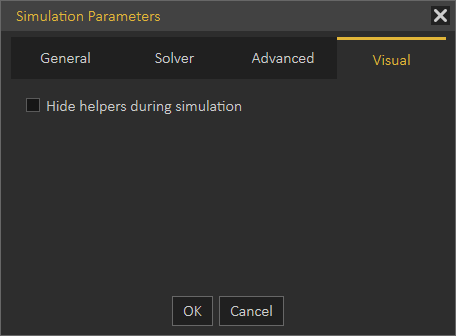
- The Visual Tab includes the following setting fields, as shown in the following image:
Collision
Enable All: This toggle button allows you to choose one of two predefined options (Enable All and Disable All). The icon of which changes with each click and cycles between two states; the currently displayed value presents the state which will be applied if the user clicked it. By default, collision is disabled.
SimLab Composer allows you to enable and disable each Solid individually by using its independent Solid Properties Panel.
Post Processing

To Animation: The To Animation button automatically exports the simulation results of the latest simulation session as an animation in the Animation Workbench.
Interactive Menu
Simulation mode has been developed for real-time interactive simulation. The new version of SimLab Composer takes Simulation to the next level, interactive simulation was added to allow the user to control machines using a Keyboard, or a Joystick.
It is designed to work with the Xbox One Controller, and the possibility to work with other game controllers such as the PS3 game controller.
Tutorial for VR Interactive Simulation:
Start/Stop Group
You can start or stop the run of an interactive simulation by clicking over the Start/Stop button (as shown in the following image):
- Start/Stop: Either start or stop the Interactive Simulation.
Interactive Simulation supports pointer devices, sliders, keyboards, and joysticks.
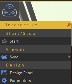
Design Group
- Design Panel: A button that launches the Interactive Physics Entities dialog box.
- Parameters: A button that launches the Simulation Parameters dialog box.
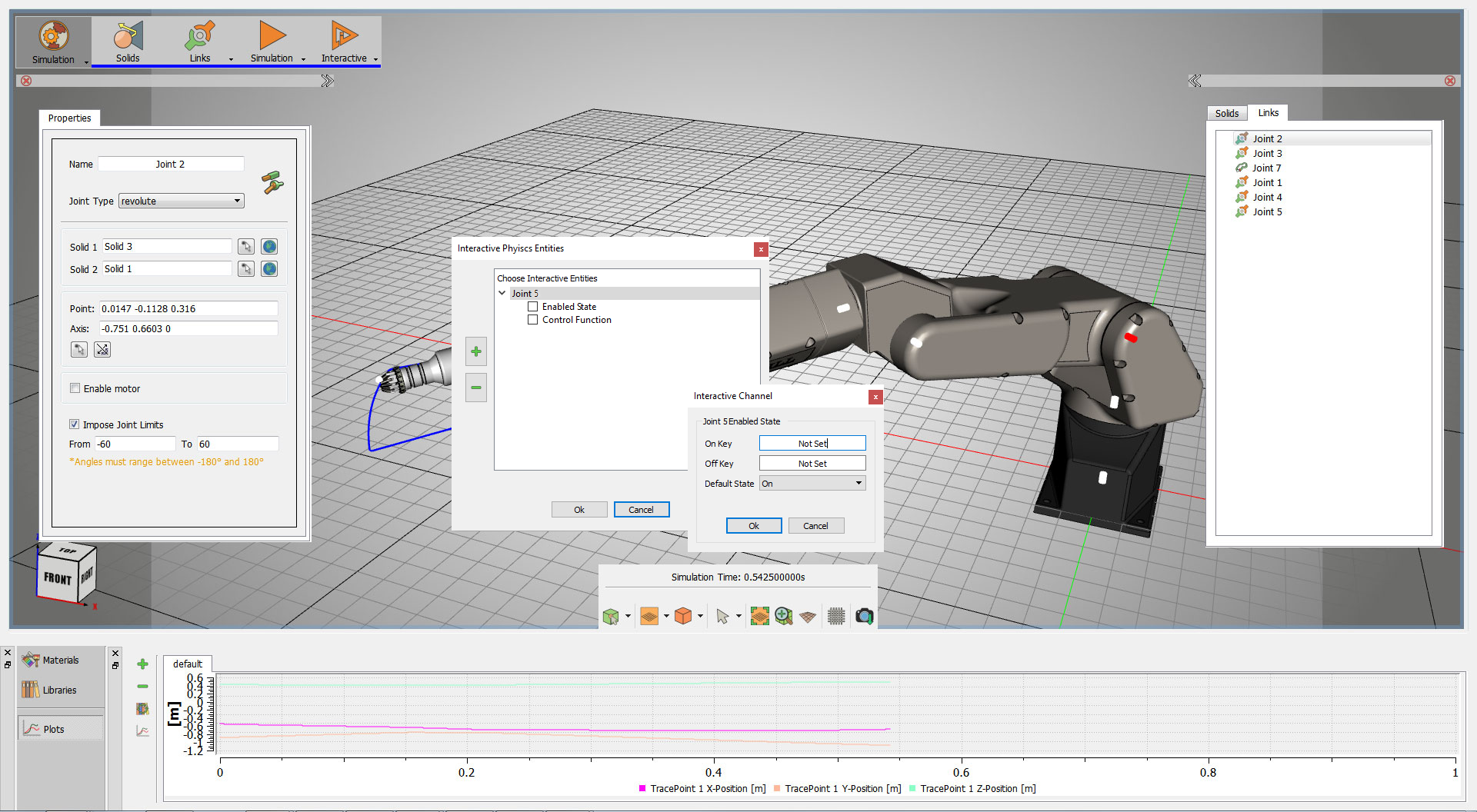
The Design Tab includes the following setting fields, as shown in the following image:
 Plus: Click it then choose a solid from the Solids Menu to add it.
Minus: Remove an entity from this list.
OK: To confirm and accept settings.
Cancel: To abort the operation.
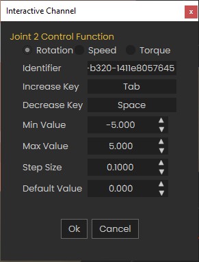
Control Function
- Rotation
- Speed
- Torque
- Identifier (necessary for executing interactive simulations via a WebSocket server)
- Increase Key
- Decrease Key
- Min Value
- Max Value
- Step Size
- Default Value
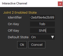
Control State
- Identifier (necessary for executing interactive simulations via a WebSocket server)
- On Key
- Off Key
- Default State
The interactive Simulation Parameter dialog box appears when the Parameters button is clicked. This dialog box is a preference panel containing multiple panels, using tabs as a navigational widget for switching among three sets of settings. The tabs are General, Solver, Advanced and Visual.
The Simulation Parameters dialog box is the same as the Simulation Parameters dialog box found in the Simulation Tab except for the General tab.
Interactive Simulation supports pointer devices, sliders, keyboards and joysticks.
Forward (Support Sliders, Keyboard, and Console Controller)
The Interactive mode for simulation supports game controllers in addition to the standard input peripherals.
The Xbox One Controller is the primary controller for Microsoft Xbox One console. The Xbox One Controller is powered by 2 AA batteries, however, the Micro USB port can be used to power the controller, instead of its wireless connectivity.
 (the Microsoft Xbox One controller)
Also, the Sony PS3 Controller is the primary controller for Sony Playstation 3 console. The Sony Playstation Controller features an internal built-in battery, however, the USB mini-B to USB-A cable can be used to connect the controller to the PC by wire instead of its independent Bluetooth connection.
 (Sony Playstation controller)
SimLab Composer offers direct support for the controller of Microsoft Xbox one. On the other hand, the controller of Sony PS3 requires third-party software to work properly with SimLab Composer on a PC. For more information, contact us at (support@simlab-soft.com)
Through GUI (Slider Bars)
The horizontal slider lets you set or adjust a value by moving an indicator. This control is a horizontal slider with a handle that can be moved right and left on a bar to select a value. The bar allows you to make adjustments to rotation or speed values throughout a range of pre-defined values. It allows you to alter the movement speed while being in the scene by decreasing it by dragging to the left (Slower) or increasing it by dragging it to the opposite direction (Faster).
Controller sticks are sensitive. So take advantage of this property when designing a panel of increase and decrease keys for the interactive entities for controlling control functions
Plotting Library
For the purpose of simulation data analysis and post-processing, the user can use this graphical technique for representing a simulation data set as a graph, showing the relationship between two or more variables. The visual presentation of different functions is very useful for users who can quickly derive an understanding as a short path to gain insight in terms of testing assumptions, model selection, relationship identification, factor effect determination, etc. as shown in the following image a Plotting Area of two graphs.
The panel of the Plotting Library is located vertically on its left side, presenting the following four buttons:

- Add New Plot Tab: This button allows the user to add a new plot tab to Plotting Library.
- Delete Current Plot Tab: This button allows the user to delete the activated Plot Tab.
- Manage Library: The user can add multiple graphs assigned to present the desired simulation data. Four types of chart formation are available, as shown in the following image Single Plot, Dual Vertical Plots, Dual Horizontal Plots, and Four Plots.
- Manage Curves: This launches the Manage Curves dialog box, letting the user plot selected channel(s) on the desired graph area.
The Plotting Area is only associated with the Simulation Tab, it appears at the bottom of the Simulation Workbench once the Simulation Tab is activated.
Co-Simulation
The Co-Simulation menu provides users with various options to facilitate simulation tasks. Below are the options available in this menu:
-
Open/Close Server
-
Use this option to open or close the local WebSocket server dedicated to passive and interactive real-time simulation. WebSockets enable two-way interactive communication sessions between a client application (SimLab VR Viewer or a web client) and a local host (SimLab Composer).
-
-
Export VR Package
-
This option allows you to export the current simulation as a simulation-compatible VR Package.
-
-
Simulation Sub-Menu

-
Desktop
-
Simulate in SimLab VR Viewer using desktop mode.
-
-
VR
-
Simulate in SimLab VR Viewer using virtual reality mode (VR headset).
-
-
Start Simulation
-
Initiate the simulation process using the local WebSocket server.
-
-
-
Interactive Sub-Menu

-
Desktop
-
Interact with the simulation in SimLab VR Viewer using desktop mode.
-
-
VR
-
Interact with the simulation in SimLab VR Viewer using virtual reality mode (VR headset).
-
-
Start Simulation
-
Start interactive simulation using the local WebSocket server.
-
-